
Sometimes, when we have a lot of data, or we want to import some data from somewhere else to use it ourselves, lists and dictionaries just don't cut it.
They look clunky and ugly. I think we should learn something that can make them look better and also allow us to do fun stuff with them, like plotting them on graphs and such!
Pandas is a library in Python that allows us to do this. To start with, we'll import our pandas library into our python installation so we can play around with it:
pip install pandas
Now we have it! If we open up a new file, we can start the file off by importing our library:
import pandas as pd
You don't have to import it as pd, but it'll help as a lot of future tutorials you'll see elsewhere on the internet will use pd as the way to reference pandas, so it's handy for us to do it like this too.
So we have pandas, and we've imported it. Now we need some data to play around with. You can copy and paste this code to save you from having to type it yourself, so we can take a look at it.
import pandas as pd

# create a dictionary of data
data = {'name': ['John', 'Jane', 'Jim', 'Joan'],
        'age': [32, 28, 41, 35],
        'country': ['USA', 'UK', 'Canada', 'Australia']}

# create a pandas data frame from the dictionary
df = pd.DataFrame(data)

# view the data frame
print(df)
So. We create a dictionary of data, this should be fairly obvious to visualise in our minds.
We then create what's called a DataFrame. This is how pandas holds onto the data. It's like a little box the panda uses to hold all our data.

Our final command just prints the DataFrame out for us.
   name  age   country
0  John   32        USA
1  Jane   28         UK
2   Jim   41     Canada
3  Joan   35  Australia
You'll notice how it also makes it look nice and tidy. It has created the first column for us, which is how pandas indexes the data. It's how we will refer to it in future if we need to work with it by index.
What can we do with the data?
One thing we can do is sort it by Age, if we wanted to for any reason. The way to do this would be:
df.sort_values(by='Age', ascending=True, inplace=True)
Pretty simple, we could do this in descending order too.
You'll notice a command inplace=True there. This is done because if we didn't specify that, pandas would want to create a new dataframe with the edited data. We just want to edit the one we have.
Now, the data looks like this:
   Name  Age    City
2   Jim   28   Paris
0  John   32  New York
1  Jane   45   London
3  Joan   51   Berlin
You'll notice the indexes are all mixed up though! That's because as far as pandas is concerned, it still wants to remember the index of the items you put in. If we wanted to get back to where we were before, we would do this:
df.sort_index(ascending=True, inplace=True)
And that's it! I love how Python most commonly has commands that make sense how you use them.
CSV files
Let's use it on something a bit more complex so we can see how powerful it is.
When you commonly have spreadsheets of data to work through, that you have created yourself or that you have exported from somewhere else, you can use Pandas to process that data yourself, so you know how its being used.
CSV files are Comma Seperated Values files that, when opened in a text editor, look like this:
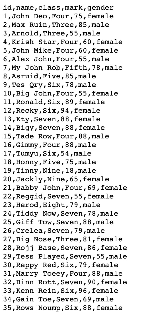
It's as it says - they are values separated by commas. Let's now do something with this.
I saved this file on my PC as student.csv. Once done, I put it in the same directory as my program, and then used pandas to import that CSV file like this:
import pandas as pd

# read a CSV file and store it as a data frame
df = pd.read_csv("student.csv")

# view the data frame
print(df)
When it's printed on that bottom line, it'll look like this:
    id         name  class  mark  gender
0    1     John Deo   Four    75  female
1    2     Max Ruin  Three    85    male
2    3       Arnold  Three    55    male
3    4   Krish Star   Four    60  female
4    5    John Mike   Four    60  female
5    6    Alex John   Four    55    male
6    7  My John Rob  Fifth    78    male
7    8       Asruid   Five    85    male
8    9      Tes Qry    Six    78    male
9   10     Big John   Four    55  female
10  11       Ronald    Six    89  female
11  12        Recky    Six    94  female
12  13          Kty  Seven    88  female
13  14         Bigy  Seven    88  female
14  15     Tade Row   Four    88    male
15  16        Gimmy   Four    88    male
16  17        Tumyu    Six    54    male
17  18        Honny   Five    75    male
18  19        Tinny   Nine    18    male
19  20       Jackly   Nine    65  female
20  21   Babby John   Four    69  female
21  22       Reggid  Seven    55  female
22  23        Herod  Eight    79    male
23  24    Tiddy Now  Seven    78    male
24  25     Giff Tow  Seven    88    male
25  26       Crelea  Seven    79    male
26  27     Big Nose  Three    81  female
27  28    Rojj Base  Seven    86  female
28  29  Tess Played  Seven    55    male
29  30    Reppy Red    Six    79  female
30  31  Marry Toeey   Four    88    male
31  32    Binn Rott  Seven    90  female
32  33    Kenn Rein    Six    96  female
33  34     Gain Toe  Seven    69    male
34  35   Rows Noump    Six    88  female
As before, we can use the power of the Panda to sort this data for us - I want to sort this by gender, so I can see all the males together and all the females together.
df.sort_values(by="gender", inplace=True)
And the result:
    id         name  class  mark  gender
0    1     John Deo   Four    75  female
32  33    Kenn Rein    Six    96  female
31  32    Binn Rott  Seven    90  female
29  30    Reppy Red    Six    79  female
27  28    Rojj Base  Seven    86  female
26  27     Big Nose  Three    81  female
21  22       Reggid  Seven    55  female
20  21   Babby John   Four    69  female
19  20       Jackly   Nine    65  female
13  14         Bigy  Seven    88  female
12  13          Kty  Seven    88  female
34  35   Rows Noump    Six    88  female
10  11       Ronald    Six    89  female
9   10     Big John   Four    55  female
3    4   Krish Star   Four    60  female
4    5    John Mike   Four    60  female
11  12        Recky    Six    94  female
1    2     Max Ruin  Three    85    male
2    3       Arnold  Three    55    male
30  31  Marry Toeey   Four    88    male
28  29  Tess Played  Seven    55    male
5    6    Alex John   Four    55    male
25  26       Crelea  Seven    79    male
24  25     Giff Tow  Seven    88    male
23  24    Tiddy Now  Seven    78    male
6    7  My John Rob  Fifth    78    male
7    8       Asruid   Five    85    male
8    9      Tes Qry    Six    78    male
18  19        Tinny   Nine    18    male
33  34     Gain Toe  Seven    69    male
16  17        Tumyu    Six    54    male
15  16        Gimmy   Four    88    male
14  15     Tade Row   Four    88    male
22  23        Herod  Eight    79    male
17  18        Honny   Five    75    male
They are sorted female first because female is first in the alphabet. Likewise, we can sort by mark too, in descending order, to see who got the highest and lowest:
df.sort_values(by="mark", ascending=False, inplace=True)
Result:
    id         name  class  mark  gender
32  33    Kenn Rein    Six    96  female
11  12        Recky    Six    94  female
31  32    Binn Rott  Seven    90  female
10  11       Ronald    Six    89  female
12  13          Kty  Seven    88  female
13  14         Bigy  Seven    88  female
30  31  Marry Toeey   Four    88    male
34  35   Rows Noump    Six    88  female
24  25     Giff Tow  Seven    88    male
15  16        Gimmy   Four    88    male
14  15     Tade Row   Four    88    male
27  28    Rojj Base  Seven    86  female
7    8       Asruid   Five    85    male
1    2     Max Ruin  Three    85    male
26  27     Big Nose  Three    81  female
25  26       Crelea  Seven    79    male
22  23        Herod  Eight    79    male
29  30    Reppy Red    Six    79  female
8    9      Tes Qry    Six    78    male
6    7  My John Rob  Fifth    78    male
23  24    Tiddy Now  Seven    78    male
0    1     John Deo   Four    75  female
17  18        Honny   Five    75    male
33  34     Gain Toe  Seven    69    male
20  21   Babby John   Four    69  female
19  20       Jackly   Nine    65  female
4    5    John Mike   Four    60  female
3    4   Krish Star   Four    60  female
5    6    Alex John   Four    55    male
28  29  Tess Played  Seven    55    male
2    3       Arnold  Three    55    male
9   10     Big John   Four    55  female
21  22       Reggid  Seven    55  female
16  17        Tumyu    Six    54    male
18  19        Tinny   Nine    18    male
Okay, so that's all well and good, but it's not pretty is it?
Well, no. It's still a bit boring. Let's make some nice graphs of it all so the panda is happy!
I downloaded a CSV file from a datasets website (comment if you'd like to know from where!) with the Global Temperatures of the planet for the last roughly 270 years.
I then imported it, like before, as such:
import pandas as pd

df = pd.read_csv('temps.csv')
I won't print out the entire file - it's roughly 3200 rows. All I'm interested in is graphing this data to see how it looks!
First though, we need to add a new library as pandas can't plot data. Type the following in your command prompt/terminal to install a library called matplotlib:
pip install matplotlib
Now, we can use matplotlib like we used pandas:
import matplotlib.pyplot as plt
As before, rather than typing out that complex matplotlib.pyplot every time, we use plt for our ease and, again, because that's the general way it's done online.
I then added this code to the file:
plt.plot(df['dt'], df['LandAverageTemperature'])

plt.title('Average Land Temperature')

plt.xlabel('Year')
plt.ylabel('Temperature (Celsius)')

plt.show()
So, in this bit of code, we:
Tell matplotlib the 2 columns to plot - 'dt' is our Year, and 'LandAverageTemperature' is the temperature on that year.
Add a title
Add an x (horizontal) label of 'Year'
Add a y (vertical) label of 'Temperature (Celsius)'
Show the plot
Everything should now have worked and you'll see a pretty crazy jagged line on your screen like this:
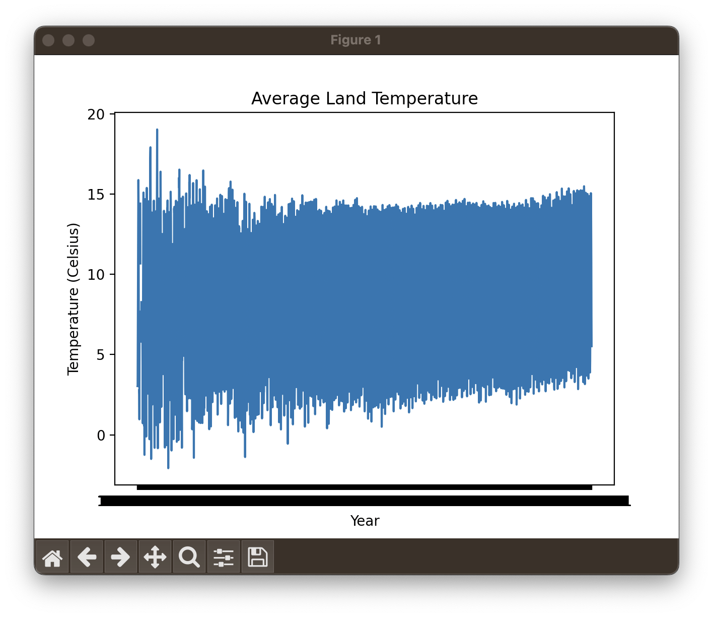
It looks so messy because we have 3200 plots here - smaller dataframes wouldn't use so many plots but this is just an example.
Phew - that was a lot! Now to summarise:
Pandas is a useful library to arrange our complex data, manually that we put in, or through a CSV file, into a nice looking box of data to play around with
We know how to sort the data by certain columns
We imported matplotlib to actually plot our data to help us visualise it easier.
We plotted the data and could label the created plot so we can understand the visualisation.
I hope you all had fun learning this! It was a lot so don't worry if you need to read through it over and over.
Please comment if you need any further advice or anything, I love seeing your comments and thank you to all the subscribers! I hope to bring you constant content to keep you all learning. Remember - the more we learn, the more capable we are to learn.